Regressions are
parametric models that predict a quantitative outcome (dependent variable) from
one or more quantitative predictor variables (independent variable). The model
to be applied depends on the kind of relationship that the variables exhibit.
Regressions take the form
of equations in which “y” is the response variables that represent the outcome
and “x” is the input variable, that is to say the explanatory variable. Before
undertaking the analysis, it is important that several conditions are met:
- -
Y values
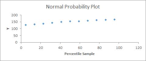
must have a normal distribution: this can be analyzed with a standardized
residual plot, in which most of the values should be close to 0 (in samples
larger than 50, this is less important), or a probability residual plot, in
which there should be an approximate straight line (Figure 31);
- -
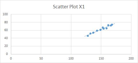
Y values
must have a similar variance around each x value: we can use a best-fit line in
a scatter plot (Figure 32);
- -
Residuals
must be independent; specifically, in the residual plot (Figure 33), the points must be equally distributed
around the 0 line and not show any pattern (randomly distributed).
Figure
31: Normal Probability Plot
Figure
32: Best-Fit
Line Scatter Plot
If the conditions are
not met, we can either transform the variables
or perform a non-parametric analysis (see 47. INTRODUCTION TO NON-PARAMETRIC MODELS).
In addition,
regressions are sensitive to outliers, so it is important to deal with them
properly. We can detect outliers using a standardized residual plot, in which data
that fall outside +3 and -3 (standard deviations) are usually considered to be
outliers. In this case we should first check whether it was a mistake in
collecting the data (for example a 200-year-old person is a mistake) and
eliminate the outlier from the data set or replace it (see below how to deal
with missing data). If it is not a mistake, a common practice is to carry out
the regression with and without the outliers and present both results or to
transform the data. For example, we may apply a log transformation or a rank
transformation. In any case we should be aware of the implications of these
transformations.
Figure
33:
Standardized Residuals Plot with an Outlier
Another problem with regressions
is that records with missing data are excluded from the analysis. First of all we
should understand the meaning of a missing piece of information: does it mean 0
or does it mean that the interviewee preferred not to respond? In the second
case, if it is important to include this information, we can substitute the
missing data with a value:
- -
With
central tendency measures, if we think that the responses have a normal
distribution, meaning that there is no specific reason for not responding to
this question, we can use the mean or median of the existing data;
- -
Predict
the missing values using other variables; for example, if we have some missing
data for the variable “income,” maybe we can use age and profession to for the prediction.
Check the linear
regression template (see 38.
LINEAR REGRESSION), which provides an example of how to generate
the standardized residuals plot.


