77. MONTE CARLO SIMULATIONS

OBJECTIVE

Determine probable outcomes.

DESCRIPTION

In deterministic models we predict events in a simple linear system and we assume that the initial conditions do not change. Besides, the same initial conditions will give the same results. However, the world is more complicated and events are usually determined by a complex interrelation of different variables, some of which are difficult or almost impossible to estimate. Monte Carlo simulations solve this problem by using probability distributions for each input variable and then running several simulations to produce probable outcomes. We can say that this model allows the prediction of an outcome without conducting many expensive experiments.

The steps for performing a Monte Carlo simulation are:

• -          Define the mathematical formula for the outcome;
• -          Identify the probability distributions of the input variables and define their parameters;
• -          Run the simulations;
• -          Analyze and optimize.

Monte Carlo Simulation Output

Input and Output Variables

The first step in a Monte Carlos simulation is to define the output, that is to say to identify the variable that we want to predict, for example “profits.” Then we should identify the input variables on which “profits” depend. Some of them may be certain; for example, we can have a fixed cost with a specific value, but usually they are uncertain. For each of the uncertain variables, we need to identify a specific probability distribution to use for the simulation. Examples of distribution are:

• -       Discrete distribution: we define the probability of a finite number of values;
• -    Uniform distribution: each variable value has similar probabilities (for example, when throwing a die, each number has a 1/6 probability);
• -       Bernoulli distribution: we have only two alternative and exclusive outcomes (0 or 1);
• -     Normal distribution: the central values are the most probable ones (defined by the mean and standard deviation);
• -       Triangular distribution: we have a most probable value and a lower and an upper limit;
• -        Other distributions: exponential, logarithmic, binomial, beta, etc.

Having identified the distribution, we can use a chi-square test (see 48. CHI-SQUARE) to check whether the data fit the chosen distribution. An alternative would be to conduct a Korm–Smirnov test.

In this phase we also write the mathematical formula by which the outcome is defined, for example:

Profits = (Price – Variable cost) * Units – Fixed Costs

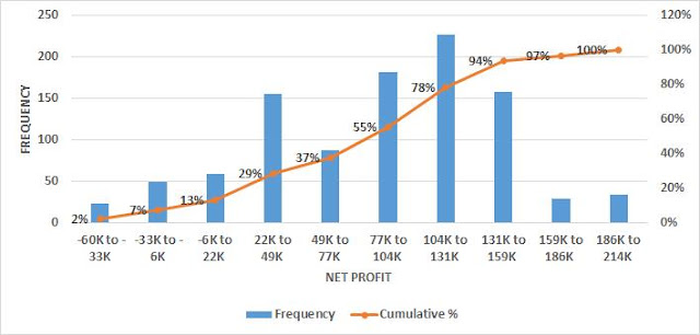
The simulation is then performed repeating the input variables (with each specific probability distribution) hundreds or thousands of times to obtain a distribution of probable results.

Analysis and Optimization

Once the range of probable results has been obtained, depending on the objective, we use indicators such as the minimum value, maximum value, average, standard deviation, and so on. In general we usually compare:

• -        Expected value: the mean of all the outputs with its confidence intervals;
• -       Risk: in the proposed example it is the probability of negative profits (% of outputs < 0), but we can also choose a specific value.

It is also possible to compare different simulations with different input variables’ values or distributions. To compare them, we should calculate the confidence intervals of both expected values and risks. If the range between the confidence intervals does not overlap, we can infer that one scenario is better or worse than the other one.

If the objective is to use the results for a business plan or in risk analysis, we can stop here, but if we want to optimize the outcomes, a sensitivity analysis is needed. In this kind of analysis, we measure the “importance” of each input and may decide to act on the most influential ones. Usually the correlation coefficient between each input and the output is used, but different techniques can be adopted.

TEMPLATE

Discount code -40%: BLOG_ANALYTICS_MODELS